Ian Fairchild, Alejandro Cearreta, Colin Summerhayes, Agnieszka Gałuszka, Michael Wagreich

The Anthropocene Working Group is preparing the case for the definition of a new stratigraphic Epoch: this requires the demonstration of an objective change in properties of a geological archive over time. As each property being examined for this distinction can be considered as a time series, we encounter a classic scientific problem of distinguishing signal from noise. We need to understand the reasons why a signal of change should exist in order to know how to look for it—for example, in what chemical form would a new pollutant emerge? We also need a theory (a model) of the noise—over time, how large are the natural background fluctuations, and what are their properties? A familiar example of this challenge is the tricky problem of distinguishing long-term climate change from the background of weather events. In this essay we examine these issues with respect to several chemical signals of environmental change which reflect global (anthro-)(bio-)geochemical cycles. To begin, we see what can be learned from the extensive measurements of sea-level change: an instructive example of a high-quality source of data with considerable noise in terms of geographic variation.

Variations across time and space: Sea-level change

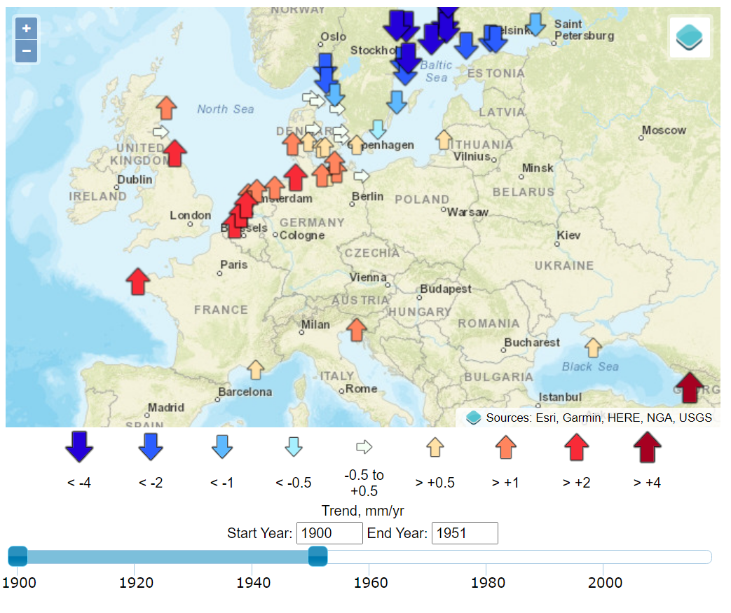
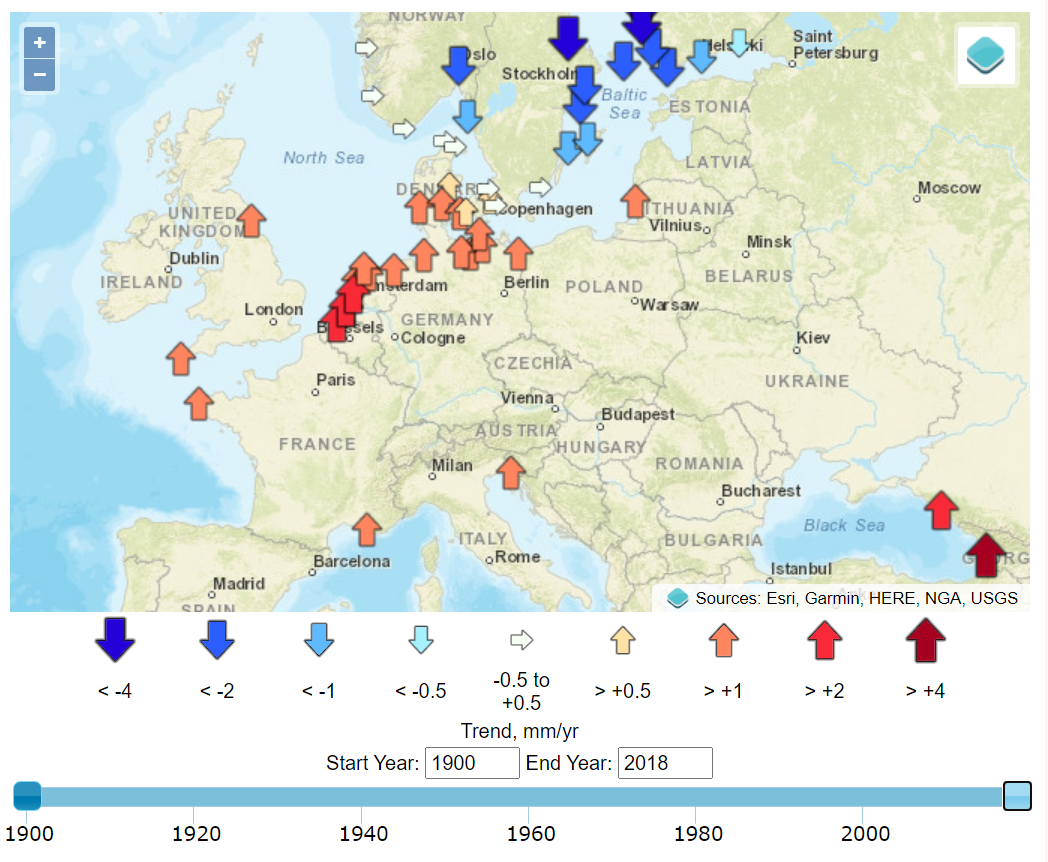
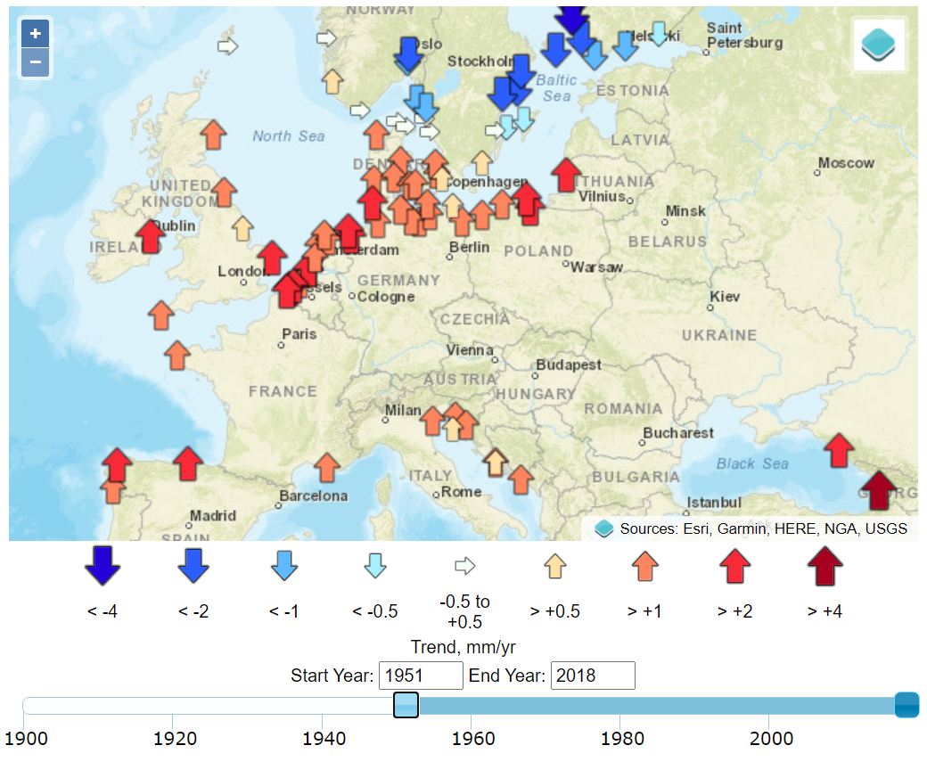
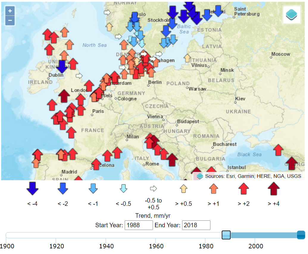
Today, much of the world’s human population lives in the coastal areas at densities about three times higher than the global average. As these coastal environments are extensively reclaimed for agriculture, urbanization, and industry, sea-level rise is an existential threat to many communities. Systematic observations of the height of water at the coastline began in Amsterdam in 1682 and computations of mean sea level became possible when automatic tide gauges, which allowed continuous water height measurements, were invented in the 1930s. Sea level at a given location represents the mean height of the water surface relative to the underlying geological substrate. Establishing this mean requires time-averaging myriad fluctuations related to climatic and geophysical factors.11Valérie Masson-Delmotte, Michael Schulz, Ayako Abe-Ouchi, Jürg Beer, Andrey Ganopolski, Jesus Fidel González Rouco, Eystein Jansen, Kurt Lambeck, Jürg Luterbacher, Tim Naish, Timothy Osborn, Bette Otto-Bliesner, Terrence Quinn, Rengaswamy Ramesh, Maisa Rojas, Xue Mei Shao, and Axel Timmermann, “Information from Paleoclimate Archives,” in Climate Change 2013: The Physical Science Basis. Contribution of Working Group I to the Fifth Assessment Report of the Intergovernmental Panel on Climate Change , ed. Thomas F. Stocker, Dong Quin, Gian-Kasper Plattner, Melinda Tignor, Simon K. Allen, Jonas Boschung, Alexander Nauels, Younan Xia, Younan Xia, V. Bex and Pauline M. Midgley. Cambridge, UK: Cambridge University Press, 2013: pp. 383–464, https://www.ipcc.ch/site/assets/uploads/2018/02/WG1AR5_Chapter05_FINAL.pdf. Tides, for example, display a range of variabilities on longer timescales than the familiar diurnal variation, and year-to-year variations in storminess can be significant sources of noise. While tide gauges provide data that is highly precise and accurate in relation to time and space, their signal is local, and as we examine below, their noise is related to geographic variations.

To understand sea level prior to the late twentieth century when tide gauges were widespread, we must use geological data. Salt marsh sediments contain microfossils whose narrow height distribution within the tidal range is delimited by modern studies. The sediments can be dated by radiometric analyses (¹⁴C, ²¹⁰Pb) and the use of stratigraphic markers of pollutants, including metals, rare isotopes from atmospheric nuclear test measurements, and human-made pollutants. The resulting records of a proxy for sea level have a precision of ±5 years in the twentieth century and a vertical resolution within ±5 cm.22Colin Summerhayes and Alejandro Cearreta, “Climate Change and the Anthropocene” in The Anthropocene as a Geological Time Unit, eds. Jan Zalasiewicz, Mark Williams, Colin Waters, and Colin Summerhayes. Cambridge, UK: Cambridge University Press, 2019, pp. 200–241.

The primary anthropogenic disturbance to the pre-existing long-term trends in sea level is the emission of greenhouse gases. Since the mid-twentieth century, 90 percent of all carbon used to date by humans was consumed to drive the huge recent industrial development.33Jaia Syvitski, Colin N. Waters, John Day, John D. Milliman, Colin Summerhayes, Will Steffen, Jan Zalasiewicz, Alejandro Cearreta, Agnieszka Gałuszka, Irka Hajdas, Martin J. Head, Reinhold Leinfelder, John McNeill, Clément Poirier, Neil L. Rose, William Shotyk, Michael Wagreich, and Mark Williams, “Extra-ordinary Human Energy consumption and Resultant Geological Impacts Beginning Around 1950 CE Initiated the Proposed Anthropocene Epoch,” Communications Earth & Environment, vol. 1 (2020): pp.1–13, https://www.researchgate.net/publication/344685697_Extraordinary_human_energy_consumption_and_resultant_geological_impacts_beginning_around_1950_CE_initiated_the_proposed_Anthropocene_Epoch. Consequently, the lower atmosphere warmed 1.2°C, the ocean increased its temperature, most mountain glaciers are retreating, and both the Antarctic and Greenland ice sheets are losing mass: accordingly, the global sea level rose 30 cm.44Colin Summerhayes and Alejandro Cearreta, “Climate Change and the Anthropocene.” Sea-level change is one of the most important consequences of the Quaternary (last 2.6 million years) climate variability, as the sea level decreases during glacial intervals and increases during interglacial phases. Comparing the tide-gauge and geological records shows that the speed of recent sea-level rise in the post-glacial interval has recently increased. Relatively low global rates of increase during the last 7,000 years (average <1 mm/year) transitioned upwards in the twentieth century and are currently >3 mm/year.55Valérie Masson-Delmotte et al., “Information from Paleoclimate Archives.” Global average sea levels are currently higher than at any time in the last 115,000 years, after the end of the previous interglacial phase.

We now know the direct causes of this change precisely because of the advent of satellite monitoring complemented by accurate surface devices (such as autonomous floats) in the ocean. Measurements of the absolute height of the ocean surface began with the launch of TOPEX/Poseidon in 1992, and were later enhanced by the GRACE satellite mission, which uses measurements of gravity to understand ice mass loss from ice sheets and glaciers. The absolute contribution of melting of the Greenland and Antarctic ice sheets to sea-level rise has increased since the early 1990s while expansion of the surface layer of the ocean due to warming has also accelerated.66Hans-Otto Pörtner, Debra C. Roberts, Valérie Masson-Delmotte, and Panmao Zhai, “IPCC, 2019: IPCC Special Report on the Ocean and Cryosphere in a Changing Climate,” 2019, https://www.ipcc.ch/site/assets/uploads/sites/3/2019/12/SROCC_FullReport_FINAL.pdf.

The timing of the measured sea-level inflections matches, with a delay of about a decade, the stepped changes in atmospheric carbon dioxide concentrations.77Colin Summerhayes and Alejandro Cearreta, “Climate Change and the Anthropocene.” Additional noise in the time domain of the calculated global mean trends of sea level is observed to coincide with volcanic eruptions (negative deviations) and the 2016 Super El Niño and 2011 La Niña events (positive and negative deviations, respectively), as can be seen in the Global Mean Sea Level chart provided by the University of Colorado. Other processes, such as ocean dynamics, tectonics, or glacial isostatic adjustment are spatially variable and cause sea-level rise to vary (usually very slowly) in rate and magnitude between different regions. Local and regional changes in these climatic and geophysical factors produce significant deviations from a global average rate of sea-level change.88Valérie Masson-Delmotte et al., “Information from Paleoclimate Archives.” These dynamics are well illustrated by the interactive graphics at the Permanent Service for Mean Sea Level (PSMSL) based at the National Oceanography Centre in Liverpool.

Europe is a continent well-furnished with tide gauges since the beginning of the twentieth century. Their data reveal large regional variations, primarily associated with rising land in Scandinavia where rebound effects from the last ice age are still in progress. Using data from recent decades, the reduction in sea-level fall in these areas and the increase in rise elsewhere is clear. By contrast, Australia’s trends in the early decades of the twentieth century cannot be reliably established because of the lack of monitoring sites. However, over the last three decades, the rising trend is unequivocal, including in areas such as coastal South Australia which are characterized by long-term uplift of the land.

The latest IPCC projections (2019) predict an average rise in the sea level at the end of the twenty-first century of 28–57 cm in a scenario of drastic reduction in greenhouse effect emissions, and of 55–140 cm if there is growth in emissions (see below). The spread within the forecasts reflects the uncertainties that exist about the future behavior of the Antarctic and Greenland ice sheets.

Climate signals in ice cores: Oxygen and hydrogen isotopes

Certain elements and their isotopes (atoms of the same element differing in mass) can be used as geochemical tracers of anthropogenic impact. Our understanding of the extent to which ice sheets have waxed and waned in the past has come from the geochemistry of oxygen isotopes, originating from the work of the chemist and Nobel laureate Harold Urey in the late 1940s. Workers have traditionally used mass spectrometry to make extremely precise measurements of the ratio of abundance of a rare isotope such as ¹⁸O (spoken as oxygen-18) to a common isotope such as 16O on a gas produced in the laboratory from the material (e.g. water or calcium carbonate). The ratios are normally expressed as the delta value, e.g. δ¹⁸O, a number in parts per thousand (‰) expressing the relative abundance of ¹⁸O to ¹⁶O. Lower delta values mean both less ¹⁸O as seen in water vapor compared with its source water, and in a progressively greater lowering of ¹⁸O in rain and snow from cooling air masses. Hence ice sheets, primarily formed from evaporation from sea water, have very low delta values which, during an ice age, lead to a higher δ¹⁸O value of the remaining seawater. The larger the mass of ice, the larger this ice-volume effect. When considering oxygen in seashells, there is also a temperature effect on the composition of precipitated calcium carbonate shells which reinforces the ice-volume effect, as classically demonstrated from deep ocean cores by Sir Nicholas Shackleton in 1967. As a result, the long-term stratigraphy of the Quaternary ice ages is framed by oxygen isotope stages which alternate between cold glacial and warmer interglacial intervals, and we know that in glacial stages, the global temperature averaged 4–6°C below present values but was 9–11°C below present values in Antarctica.

Although a (small) oxygen isotope (δ¹⁸O) signal does mark the base of our current interglacial period (the Holocene) in a Greenland ice core, the subsequent variations are more subtle and below the 0.5–1°C sensitivity of the oxygen isotope proxy. Consequently, an assemblage of temperature proxies is used, rather than just oxygen isotopes, to establish Holocene temperature archives. When it comes to the mid-twentieth century proposed start for the Anthropocene, there is no discrete (δ¹⁸O) signal in oxygen isotope archives, even in the relatively sensitive Antarctic records. In fact, the gradual increase in the rate of temperature change makes it difficult to define an Anthropocene boundary on the basis of any geochemical proxy for temperature. This problem is also the basis for the struggle (now largely won) to convince politicians and the public of the reality of warming (also known as the “boiling frog syndrome” of inattentiveness to gradual risk increases).

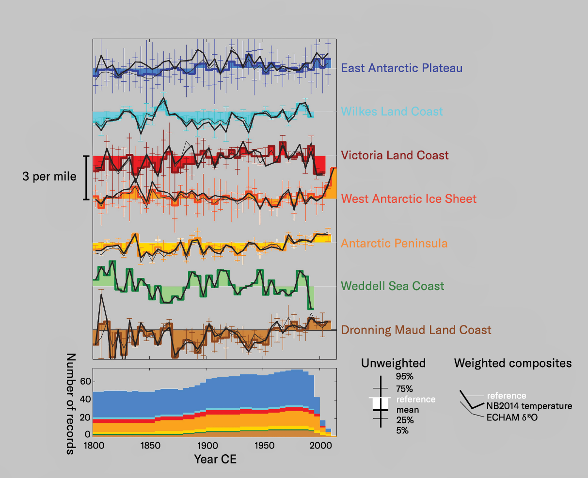
The increasing rate of change in temperature in recent decades does, however, lead to measurable changes in Antarctic ice-core records. Hydrogen isotopes show covariation with oxygen and with temperature, so measuring both elements provide a more robust measure of past temperatures. To avoid local effects, the most reliable signals are reached through the combination of multiple ice-core records from a given site and/or region, and through the site-specific calibration of the relationships between water-stable isotopes and temperature ,99Barbara Stenni, Mark A. J. Curran, Nerilie J. Abram, Anais Orsi, Sentia Goursaud, Valéire Masson-Delmotte, Raphael Neukom, Hugues Goosse, Dmitry V. Divine, Tas van Ommen, Eric J. Steig, Daniel A. Dixon, Elizabeth R. Thomas, Nancy Bertler, Elisabeth Isaksson, Alexey Ekaykin, Martin Werner, and Massimo Frezzotti, “Antarctic Climate Variability on Regional and Continental Scales over the last 2000 Years,” Climates of the Past vol. 13, (2017): pp. 1609–1634, https://cp.copernicus.org/articles/13/1609/2017/. which has been carried out under an international project identifying several discrete regions of Antarctica that exhibit somewhat different climate signals (see below). Temperature reconstructions based on the isotopic data showed warming in recent years in three of these regions. In each case the temperature increase began around 1920 and continued to the latest available measurements (ca. 2005) with rates of warming between 1 and 2°C/100 years. These increases followed substantial declines in temperature that lasted over the previous 2,000 years. However, relative to the variability of the climate signal in the rest of Antarctica for the past 2,000 years, only the rise in temperature of the Antarctic Peninsula is unusual. It seems reasonable to assume that because of its more northerly aspect, the Peninsula is subject to a slightly different climatic regime than most of the continent, and one that is closely connected to the global warming identified elsewhere on the planet. Close inspection of the isotopic temperature signal for the Peninsula suggests greater warming after about 1970 than between 1920 and 1970, much as is found in the global surface temperature signal. It seems likely, then, that the Peninsula temperature signal reflects gradual warming after 1900, followed by steeper warming after 1970, as on the rest of the globe.

The carbon cycle and sulfur in the atmosphere

A primary driver of global warming is the burning of fossil fuels which have created a first-order change in the carbon cycle. Fluxes of carbon between reservoirs have increased, and carbon, mainly as carbon dioxide, is increasingly stored in the atmosphere. This newly released carbon has a distinct fingerprint in terms of the ratio of the stable isotopes of carbon (¹³C/¹²C) as determined from mass spectrometry. Expressed in terms of the delta number (δ¹³C), the rare ¹³C is much less abundant in the biosphere (δ¹³C around -25‰), and thus in fossil fuels that stem from organic material, than in the pre-industrial atmosphere (-6.5‰). Hence atmospheric CO₂ trapped in ice cores shows an inverse relationship to δ¹³C, known as the Suess effect, with a pronounced inflection around 1965 CE. This signal in ice cores shows little noise because it reflects the composition of a well-mixed atmosphere. It therefore compares in quality with that of radioactive species such as radiocarbon and plutonium released through atmospheric nuclear tests. Carbon isotopes in other archives typically show a less clear-cut relationship because of the complexities of biochemical cycling. For example, this signal is masked altogether in cave carbonates (speleothems) because of large fractionations in carbon isotopes in cave systems. Trees provide an interesting intermediate example where, although the carbon fixed is derived directly from the atmosphere, seasonal to decadal changes in tree physiology add noise to the Suess effect. However, in the dataset shown below,1010From Neil J. Loader, Gilles Young, Håkan Grudd, and Danny McCarroll, “Stable Carbon Isotopes from Torneträsk, Northern Sweden Provide a Millennial Length Reconstruction of Summer Sunshine and its Relationship to Arctic Circulation,” Quaternary Science Reviews vol. 62, (2013): pp. 97–113, https://www.sciencedirect.com/science/article/pii/S0277379112004854?via%3Dihub#. a moving average of the data reveals the underlying atmospheric signal, with an inflection around 1960 CE. Marine records, such as from corals, also demonstrate a clear signal.

A contrasting example is provided by sulfur in the atmosphere. It is released naturally from volcanic eruptions, but emissions increased enormously because of industrial processes, particularly the burning of sulfurous coal. Because this sulfur is in the form of microscopic aerosol particles, the abundance of sulfur in geological archives and its stable isotope composition show regional variations.1111Ian Fairchild, “sulphur,” in The Anthropocene as a Geological Time Unit, eds. Jan Zalasiewicz, Mark Williams, Colin Waters, and Colin Summerhayes. Cambridge, UK: Cambridge University Press, 2019, pp. 172–178. For example, trees and speleothems in Europe show a mid-twentieth century rise followed by a fall reflecting changes in this industrial activity. These records rely on micro-scale analytical techniques at specialized facilities, such as ion probes or the fluorescence produced by X-rays in huge synchrotron facilities. Both are anthrobiogeochemical records since the O and S isotopes in sulphate in rainfall become fractionated when stored in soil humic substances. This pollution indicator is also seen as an anthrogeochemical (i.e. non-biological) signal in Greenland ice, but is absent in Antarctic ice cores.

The nitrogen cascade

The modern nitrogen cycle is a typical anthrobiogeochemical cycle because human activities have led to substantial changes in natural processes governing nitrogen fixation, its bioavailability, and its overall fate in the environment. The production of fertilizer through the synthesis of ammonia from atmospheric N₂ (Haber-Bosch process) and its use in agriculture since the beginning of the twentieth century constitute one of the most important sources of anthropogenic perturbations of the nitrogen cycle, along with the burning of fossil fuels and symbiotic nitrogen fixation by bacteria hosted by cultivated plants.

An excess of nitrogen causes a negative impact on all environmental compartments. In surface waters it brings about eutrophication, leads to a deficit in oxygen (hypoxia) in the sea, and a decreased input of dissolved silica in soils. Excessive amounts of nitrogen cause acidification and decreased biodiversity. It also diminishes the quality of air through the formation of particulate matter and ozone. The above examples of complex environmental impacts are often referred to as a “nitrogen cascade.”

Nitrogen has two stable isotopes, ¹⁴N and ¹⁵N, with ¹⁴N making up 99.63 percent of all nitrogen occurring in nature. Anthropogenic sources produce a change of nitrogen stable isotope ratios in different environmental archives. This change may potentially be used as a signal of the Anthropocene. Sample analysis is again by mass spectrometry with preparation techniques tailored to create gas for analysis from materials such as organic matter or ice. The increase in concentrations of nitrogen compounds in the environment, especially from fossil fuel burning, is usually accompanied by a decrease in δ¹⁵N values. For example, the differences in δ¹⁵N values of nitrate recorded in a Greenland ice core in the past 150 years was as high as 12‰, decreasing from +11‰ to −1‰. Similar patterns of δ¹⁵N values were found in analyses of total nitrogen in organic carbon from dated lake sediments collected from 25 remote and nutrient-poor lakes in the Northern Hemisphere. The present δ¹⁵N value of ∼8‰ recorded in North Pacific deep-sea corals is the lowest it has been during the last 5,000 years. In many environmental archives, the rate of decline in the δ¹⁵N value has accelerated and become pronounced, but there are also reports of enrichment in ¹⁵N in natural archives during recent decades. In coral skeletons from the Pearl River estuary in China, for example, relatively stable δ¹⁵N values (a range of 9 to 12‰) were recorded in the skeletons dated from the mid-Holocene to the 1980s, followed by an increase to >13‰ during 1987–1993 CE and later a decline to the pre-1980s values. The increase observed in the late 1980s/early 1990s was caused by a growing input of sewage to the Pearl River estuary (below).1212Data from Nicolas N. Duprey, Tony X. Wang, Taihun Kim, Jonathan D. Cybulski, Hubert B. Vonhof, Paul Crutzen, Gerald H. Haug, Daniel M. Sigman, Alfredo Martínez‐García, and David M. Baker, “Megacity Development and the Demise of Coastal Coral Communities: Evidence from Coral Skeleton δ¹⁵N Records in the Pearl River Estuary,” Global Change Biology vol. 26 (2020): pp. 1338–1353, https://onlinelibrary.wiley.com/doi/full/10.1111/gcb.14923; and Gordon W. Holtgrieve, Daniel E. Schindler, William O. Hobbs, Peter R. Leavitt, Eric J. Ward, Lynda Bunting, Guangjie Chen, Bruce P. Finney, Irene Gregory-Eaves, Sofia Holmgren, Mark J. Lisac, Peter J. Lisi, Koren Nydick, Lauren A. Rogers, Jasmine E. Saros, Daniel T. Selbie, Mark D. Shapley, Patrick B. Walsh, and Alexander P. Wolfe, “A Coherent Signature of Anthropogenic Nitrogen Deposition to Remote Watersheds of the Northern Hemisphere,” Science vol. 334, (2011): pp. 1545–1548, https://science.sciencemag.org/content/334/6062/1545.abstract. Nitrification (oxidation of NH₄⁺ from sewage to nitrites and nitrates) and subsequent denitrification (reduction of nitrates to N₂O and N₂) caused an increase in the δ¹⁵N values because the products of denitrification were enriched in the lighter N isotope, whereas the remaining inorganic N species were enriched in ¹⁵N. It is fortunate that despite the complexities of the biogeochemical cycling of different nitrogen species, both the nitrogen isotope records of nitrate and the organic carbon fraction reflect environmental change. The observed trends in the δ¹⁵N values of different environmental archives reflect a combination of natural- and human-driven processes, thus confirming the usefulness of stable nitrogen isotopes for our understanding of anthrobiogeochemical nitrogen cycles.

The legacy of lead

Trace metals are integral parts of natural element cycles and, before human interference, came mainly from geo-/lithogenic sources via the weathering of rocks. We focus here on lead (Pb), as it is relatively common in the Earth’s crust (average 14 ppm) compared to other trace metals, has been widely mined or formed a by-product of mining since prehistoric times, and is identified as a highly toxic element, making the monitoring of Pb contamination as well as searches for its provenance a critical issue in geological, environmental, and public research. Beginning as early as thousands of years BCE, the increased availability of anthropogenic trace metals in the environment, and thus their involvement in anthrobiogeochemical cycles, began with the mining of ores and other raw materials for use in various industrial processes: initially lead was merely a by-product, and only later was mined directly.

Many different techniques are used to determine total Pb concentrations in samples, and the analytical precision of these techniques is far less than the sample-to-sample variation. Ratios of stable isotopes such as ²⁰⁶Pb, ²⁰⁷Pb, and ²⁰⁸Pb analyzed by different types of mass spectrometry can be used to distinguish the sources of contamination by lead in the environment, e.g. in assessing the relative contributions from mining against natural background values.1313See, for example, Agnieszka Gałuszka and Michael Wagreich, “Metals,” in The Anthropocene as a Geological Time Unit, eds. Jan Zalasiewicz, Mark Williams, Colin Waters, and Colin Summerhayes. Cambridge, UK: Cambridge University Press, 2019, pp. 178–186. Natural background fluctuations vary across orders of magnitude, driven by local high-lead sources like ores, variabilities in input from weathering, and sediment dilution. Remote archives such as ice sheets largely show inputs of natural dust particles, contaminated by anthropogenic emissions such as those from lead in petrol. Because ice sheets are remote, background concentrations of Pb in Arctic and Antarctic ice cores range from a few to a few tens of parts-per thousand, whereas in other archives, such as lakes and bogs, natural background concentrations are mainly around tens of parts-per million.1414Agnieszka Gałuszka and Michael Wagreich, “Metals.”

The earliest regional to supra-regional peaks of aerosol Pb (a by-product of silver mining and smelting processes) can be identified in Northern Hemisphere ice cores from Greenland and Arctic Canada, and are linked to Phoenician-Greek mining and smelting activities some 3,000 years ago (see below). This minor peak in some environmental archives of the Northern Hemisphere was identified as a possible stratigraphic marker for an early Anthropocene.1515Michael Wagreich and Erich Draganits, “Early Mining and Smelting Lead Anomalies in Geological Archives as Potential Stratigraphic Markers for the Base of an Early Anthropocene,” The Anthropocene Review, 5, no. 2 (2018): 177–201, https://journals.sagepub.com/doi/abs/10.1177/2053019618756682

Later, silver, and thus also lead, mining and usage increased substantially during Roman times, which lead to significant human health problems. This usage is recorded in archives by a widespread lead peak, more pronounced than the earlier one, and is recognized in ice cores, estuaries, bogs, and remote lakes of the Northern Hemisphere; a Spanish source for the lead was revealed by isotope studies.1616Michael Wagreich and Erich Draganits, “Lead Anomalies in Geological Archives.”

Global lead production and usage only began to rise again with silver production in medieval times. This was followed by an even larger rise due to silver mining and production in the New World, with abundant production and use punctuated by plagues and wars. The Industrial Revolution brought a major rise in lead production and left a peak in archives around 1850–1890 CE that was much larger than the Roman peak. The Australian Broken Hill lead signal beginning around the 1850s onward formed the first peak in Antarctic ice cores. Final peak usage and global environmental contamination was reached during the mid-twentieth century, when lead was used as an antiknock additive for petrol in the increasingly fossil-fuel driven transport system. This last peak, being in several geological archives an order of magnitude higher than the former more regional peaks of lead usage, provides a marker for the Great Acceleration. Although it was not as pronounced as are other chemical markers around the 1950s, the lead peak was very distinct and globally distributed on both land and oceans. Due to the eventual recognition of its toxic behaviour, lead as a petrol additive was banned in more and more countries, starting in the USA and Europe from the 1970s onwards. The recent widespread Pb expulsion, then, began to increase in the 1920s, peaked in the late 1960s, and declined from the late 1970s onward, arriving at today’s intermediate to high values of contamination and fluxes of lead in the Earth system.1717Agnieszka Gałuszka and Michael Wagreich, “Metals.”

The Anthropocene signal amidst the noise

The large amounts of industrially-produced pollutants and emissions that have been introduced, over decades and centuries, into air, soil, and water have caused considerable changes to natural phenomena, such as the cycling of elements and changes in sea level. However, the Anthropocene signals lie amidst noise which arises for several reasons. One is the issue in making measurements with sufficient precision (easy for tide gauges, but tricky for some rare isotopes). Another is the geographic variability of many parameters. A third is the presence of natural variability over time. Despite these problems, many different types of anthropogenic signals have become increasingly prominent and isolatable since the middle of the twentieth century.

Ian Fairchild is Emeritus Professor at the School of Geography, Earth and Environmental Sciences at the University of Birmingham.

Alejandro Cearreta is Professor of Micropaleontology at the Universidad de Pais Vasco UPV/EHU, Spain, Head of the Geology Department and Director of the postgraduate program in Quaternary: Environmental Changes and Human Fingerprint.

Colin Summerhayes is Emeritus Associate at the Scott Polar Research Institute of the Geography department at the University of Cambridge.

Agnieszka Gałuszka is Full Professor at the Institute of Chemistry, of the Jan Kochanowski University in Kielce. She is an expert in geochemistry and biogeochemistry.

Michael Wagreich is Full Professor of Geology at the Department of Geology, Faculty of Earth Sciences, Geography and Astronomy, of the University of Vienna.

Cover art by Protey Temen, © All rights reserved Protey Temen